Learning R from Python

Introduction

There is always a big debate between which language, R or Python, is the best for statistical data analysis and machine learning. Both languages have pros and cons, so why not understand both? I have a strong Python background, but figured I should learn R as well. R has ggplot2, which is an amazing visualization library that seems to outdo what matplotlib and Seaborn offer through Python. Unfortunately, there seems to be a lot of information about switching from R to Python but not the other way around. So I decided to just learn R through rebuilding a Python project I have already completed.

For reference, I built a spam classifier model in Python and documented the process in a previous blog. I wanted to rebuild this spam classifier model, in a very simplified form, in R. Doing this has helped me learn many useful skills in R that I will show in this blog.

Getting Started

To begin, I downloaded Python through Anaconda. I typically code with jupyter notebooks, which come with Anaconda. I’d like to set up R in this environment as well.

First things first, let’s download R. Then in order to install properly follow the PC or Mac steps found in this helpful blog by Rich Pauloo.

Coding with R

Installing Libraries

If you need to install any of the libraries I’ll use, then you can do this with the following line of code, just change the library name:

install.packages("caret")

Importing Libraries

I’ll be using the following libraries:

library(wordcloud)
library(RColorBrewer)
library(tm)
library(magrittr)
library(caret)
library(e1071)
library(SnowballC)

Reading in the data

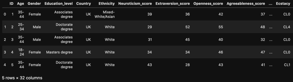
I had the spam data in a csv file from my python project, but the data originally comes from the UCI Machine Learning Repository.

I read in the data with the following code:

df <- read.csv("smsspamcollection/spamham.csv")

Data Visualizations through Wordcloud Library

Now in order to visualize the text data, I separated the data into spam vs ham (i.e. not spam) and then created a word cloud for each group. This was accomplished with the following code:

# Split dataframe by ham and spam
spam_split <- split(df, df$label)
spam <- spam_split$spam
ham <- spam_split$ham

# Create a vector of just spam text data
spam_text <- spam$text

# Create a spam corpus  
spam_docs <- Corpus(VectorSource(spam_text))

# Clean spam text with tm library
spam_docs <- spam_docs %>%
  tm_map(removeNumbers) %>%
  tm_map(removePunctuation) %>%
  tm_map(stripWhitespace)
spam_docs <- tm_map(spam_docs, content_transformer(tolower))
spam_docs <- tm_map(spam_docs, removeWords, stopwords("english"))

# Create document spam term matrix
spam_dtm <- TermDocumentMatrix(spam_docs) 
spam_matrix <- as.matrix(spam_dtm)
spam_words <- sort(rowSums(spam_matrix),decreasing=TRUE)
spam_df <- data.frame(word = names(spam_words),freq = spam_words)

# Create a vector of just ham text data
ham_text <- ham$text

# Create a ham corpus  
ham_docs <- Corpus(VectorSource(ham_text))

# Clean ham text with tm library
ham_docs <- ham_docs %>%
  tm_map(removeNumbers) %>%
  tm_map(removePunctuation) %>%
  tm_map(stripWhitespace)
ham_docs <- tm_map(ham_docs, content_transformer(tolower))
ham_docs <- tm_map(ham_docs, removeWords, stopwords("english"))

# Create document ham term matrix
ham_dtm <- TermDocumentMatrix(ham_docs) 
ham_matrix <- as.matrix(ham_dtm)
ham_words <- sort(rowSums(ham_matrix),decreasing=TRUE)
ham_df <- data.frame(word = names(ham_words),freq = ham_words)

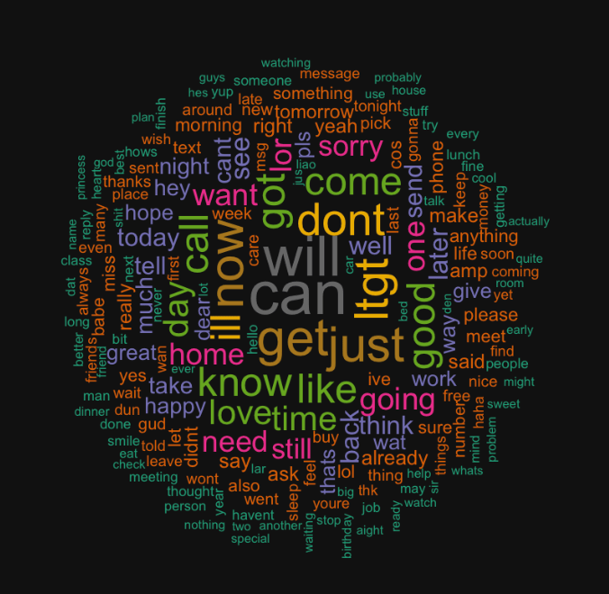
# Create spam wordcloud
wordcloud(words = spam_df$word, freq = spam_df$freq, min.freq = 1,
          max.words = 200, random.order = FALSE, rot.per = 0.35,
          colors = brewer.pal(8, "Dark2"))

# Create ham wordcloud
wordcloud(words = ham_df$word, freq = ham_df$freq, min.freq = 1,
          max.words = 200, random.order = FALSE, rot.per = 0.35,
          colors = brewer.pal(8, "Dark2"))

This code should give you two word clouds, spam and ham respectively, that look like the following:

Model Preprocessing

Now I need to do some preprocessing for the modeling. This includes creating a corpus and document term matrix, which is a sparse matrix containing all the words and the frequency of which they appear in each message. The preprocessing code also removes stop words (i.e. the, it, etc.), makes all words lowercase, finds the stem of the words, and removes punctuation and numbers.

df_corpus <- VCorpus(VectorSource(df$text))

df_dtm <- DocumentTermMatrix(df_corpus, control = 
                                 list(tolower = TRUE,
                                      removeNumbers = TRUE,
                                      stopwords = TRUE,
                                      removePunctuation = TRUE,
                                      stemming = TRUE))

I also need to train test split the data. This step is admittedly much less straightforward as compared to Python, but I was able to get it done.

# Calculate train test proportions
index <- floor(5572 * .8)

#Training & Test set
train <- df_dtm[1:index, ]
test <- df_dtm[index:5572, ]

#Training & Test Label
train_labels <- df[1:index, ]$label
test_labels <- df[index:5572, ]$label

Finally, the last step of preprocessing is converting the data into categorical data. The Naive Bayes model I am using in R requires this. This step is good practice and creating and implementing a function!

# Convert to categorical for naive bayes model
convert_values <- function(x) {
  x <- ifelse(x > 0, "Yes", "No")
}

train <- apply(train, MARGIN = 2, convert_values)
test <- apply(test, MARGIN = 2, convert_values)

Modeling

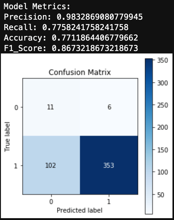
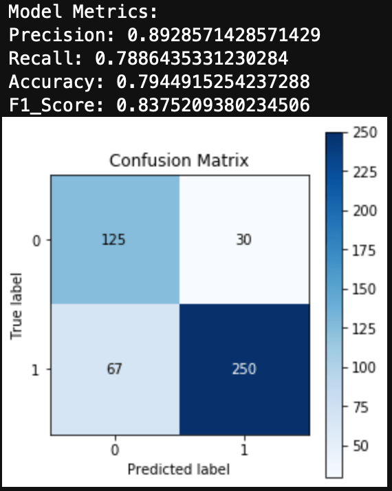
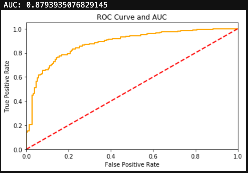
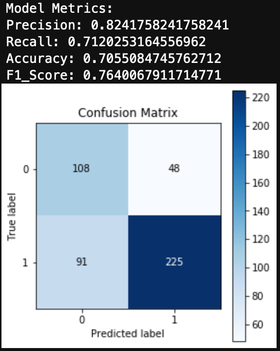
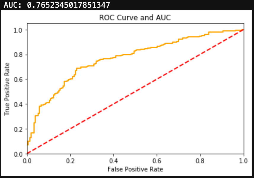
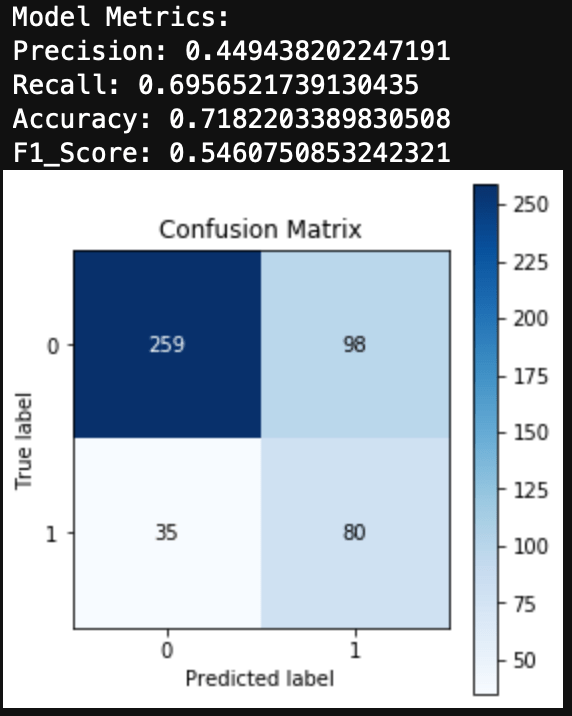
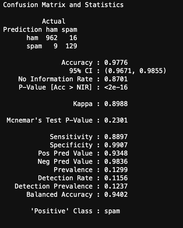
Now we can model and evaluate! The following code initiates the Naive Bayes model and computes a confusion matrix and accuracy of the Naive Bayes model on the test set of data.

#Create model from the training dataset
spam_classifier <- naiveBayes(train, train_labels)

#Make predictions on test set
y_hat_test <- predict(spam_classifier, test)

#Create confusion matrix
confusionMatrix(data = y_hat_test, reference = test_labels,
                positive = "spam", dnn = c("Prediction", "Actual"))

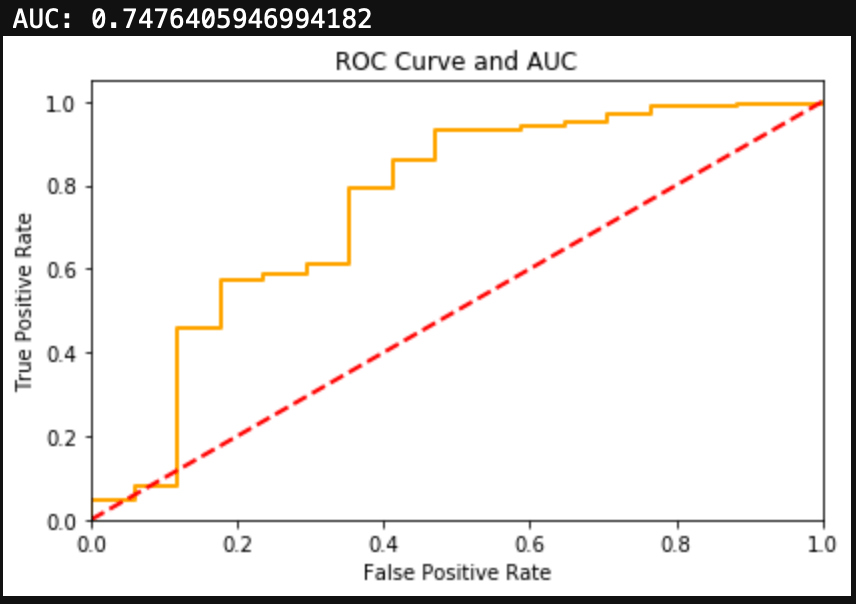
You can see the results here:

Conclusions

I was able to get a very simplified working model of my spam classifier! Although this isn’t as pretty as the model generated in Python from my previous blog, it still works and is a great success for learning R. If you are wanting to learn R from Python, I encourage you to practice R by recreating a Python project you have already created. This way you know what you want as data inputs and model outputs, and all you have to figure out is the R. Googling helps!

TensorFlow or Keras: Which is better for Neural Network Models in Python?

Introduction

As I finished up my Data Science program at the Flatiron School, I wanted to create a convolutional neural network for an image classification problem I was attempting for my capstone project. However, I wasn’t sure at first if I should use TensorFlow or Keras to build my neural network model. This lead me to writing this blog to give a general overview of the differences of TensorFlow and Keras. Hopefully this will help others avoid the same dilemma and research I went through when starting to craft my model.

TensorFlow and Keras

Both TensorFlow and Keras are frameworks to use in Python Data Science programming. Specifically, both can be applied to Deep Learning problems. Let’s look at TensorFlow first.

TensorFlow

TensorFlow is an open source project designed to help in Machine Learning. It provides a "toolbox" of resources to help craft workflows using high level APIs. You can use different levels of these APIs to accomplish different Machine Learning tasks. TensorFlow in general creates a framework that allows for easy to model building and training, as well as model deployment for all of the machine learning models generated. My personal take, however, is that TensorFlow’s model building code structure is more customizable, but more labor intensive and confusing as compared to Keras.

Keras

Keras runs on top of TensorFlow and is, in fact, a specifically designed Deep Learning wrapper of TensorFlow. It allows for quick, easy model architecture and building. Keras is also set up to run models seamlessly with both CPUs and GPUs. If you use Python, Keras will have another advantage, as it was built in Python. This makes for easier debugging. Like TensorFlow, Keras creates a framework that allows for easy model building. The code in Keras is also very consistent across different types of neural networks, which is a big advantage. Since Keras’s model building code acts like a series of building blocks, this also allows models to be improved and extended with ease. One personal take for Keras is that it also provides very clear error messages as compared to TensorFlow. It is very easy to debug your code when encountering errors while using Keras.

Recommendation

If you are someone who has very strong coding skills and wants to build an extremely customized Deep Learning model, then TensorFlow is probably the right framework to use. In all other cases, I would recommend using the Keras framework. It provides for easier coding using building blocks of code, easier debugging, and can run quicker when using GPUs.

Conclusion

Both Keras and TensorFlow are awesome frameworks to get to know for your Machine Learning needs. Remember that Keras is a framework built as a wrapper on top of TensorFlow, specifically for Deep Learning needs. TensorFlow has much more overall Machine Learning capabilities than Keras, but when it comes to building neural networks, Keras is a great framework to take advantage of.

Predicting Drug Use with Logistic Regression

Introduction

This project began as a search for classification problems to tackle. I wanted to put my classification algorithm skills to the test, but wasn’t sure what data to use for this. Luckily, after digging around on the internet for a while, I came across the UC Irvine Machine Learning Data Repository. This repository has loads of datasets and even has a feature, "Default Task", that you can toggle in order to find the common machine learning task that would be applied to a given dataset. When looking through the Classification datasets I found a dataset regarding drug use that looked interesting. The dataset was originally collected by Elaine Fehrman, Vincent Egan, and Evgeny M. Mirkes in 2015.

This dataset provides 1885 data rows, each of which represents a person. Each person has a set of demographic and personality traits alongside a set of drug use responses. Data features included things like age, ethnicity, education level, country, extraversion score, openness to new experiences score, etc… The dataset looks at 17 common drugs (including chocolate??) and how recently someone has used each of the drugs. I decided to make drug use a binary outcome by grouping no usage ever and usage over a decade ago into "non user" and all other outcomes into "user", meaning that the person has used the drug within the last decade.

At this point I decided I would use Logistic Regression to predict whether or not a person was a user of each of the 17 drugs given in the dataset. This model information could help to determine which types of people are more susceptible to certain types of drug use given their personality type and demographic traits. This information could then be used to give treatment and assistance to those who require it.

ETL

After importing the necessary libraries and loading in the dataset into a Pandas DataFrame, the raw data looks like this:

You can see that the data comes in a very weird format, but luckily there are descriptions on the data webpage. Using these descriptions, I transformed the data into a more coherent DataFrame.

Dummy Variables and Checks for Multicollinearity

After getting the data into a useful format, I needed to deal with my categorical variables. I fit dummy variables to all of them and made sure to drop one of the resulting columns. I also needed to check if any of my numeric features had multicollinearity. As you can see in the seaborn pairplot below, the only two metrics that appear to have any multicollinearity are neuroticism and extraversion, but the correlation level is below .75, so I kept both scores in the DataFrame.

DataFrame Splitting

After a little more data manipulation (changing the column order), I needed to create separate DataFrames for each drug. I decided to store each of these in a dictionary, with each key being a name for the drug DataFrame and the value being the corresponding DataFrame. This was accomplished with the chunk of code below:

Note: The above portion of the code with df.iloc[:, :34] isolates the portion of the DataFrame corresponding to the features. After column 34 are the binary drug use columns.

Helper Functions for Model Fitting

First things first, I need to import the proper libraries and functions for all the tools I’ll need for my Logistic Regression process.

A quick note on the scikitplot library. This library has many awesome functions for calculating metrics and plotting them in one step. You’ll see a use of this for confusion matrices later on.

In order to loop through my new dictionary and fit a Logistic Regression model to each DataFrame, I needed to define a few helper functions. The first function will split the DataFrame into the features and the target, X and y respectively.

The next helper function will perform standard scaling on my numeric features after I have performed a train/test split on my data.

An additional helper function I wrote performs SMOTE on the datasets. Many of the drug user datasets are very unbalanced, so in order to train my model on a balanced dataset, I need to use SMOTE to synthetically create training data points for my minority class. This function is created below.

Another useful step in Logistic Regression is using a grid search for the best performing hyperparameters C and Penalty type. These control regularization of the models and this function will output the optimized hyperparameters for each drug use model.

Finally, one last helper function. This is the function that actually fits the Logistic Regression model and creates output metrics and visualizations. This model takes in the train/test split data and the optimized hyperparameters C and Penalty type. The function when applied will create visualizations for the confusion matrix and ROC Curve. It also outputs the test sample’s class balance, which helps to inform how the test data is distributed.

Fitting the Model

Finally, it is time to fit all of the models and view the results. I wrote one last function which combines all of the above functions into one simple function that can be applied to a single DataFrame.

This function is then applied to each DataFrame in my previously created dictionary with a for loop to generate all of the necessary model results and visualizations.

Results

As there were 17 different drugs in question, I will only highlight a few of the results below. The Logistic Regression model performed well in most cases, although those with extremely unbalanced datasets performed slightly worse despite the use of SMOTE to balance the training sets.

Alcohol

Alcohol had an extremely unbalanced dataset. You can see that 96% of the test group had used alcohol. Alcohol did produce a large number of false negatives, however the F1 Score and AUC metrics signaled that this was a decent model.

Cannabis

Cannabis had a more balanced dataset than alcohol, with 67% of the test group having used the drug. The Logistic Regression for Cannabis use was able to generate both a high F1 Score and high AUC.

Nicotine

Nicotine also had a more balanced dataset than alcohol, with 67% of the test group having used Nicotine. Similarly to Cannabis, the Logistic Regression model for Nicotine was able to produce both a high F1 Score and a high AUC.

Meth

Finally, I’ll look at a drug that has an unbalanced dataset in the other direction. Obviously not a ton of people use Meth, although more than I imagined, with 24% of the test group having used Meth before. The Logistic Regression for Meth use produced a fair amount of false positives. Additionally the metrics and F1 Score are fairly low. The ROC Curve and AUC show decent results, but in the case of an unbalanced dataset, I would trust F1 Score over AUC.

Conclusions

I was able to fit a Logistic Regression model to each of the drug use DataFrames, however for some of the drugs, Logistic Regression may not be the best choice classifier model. Since a lot of the datasets are unbalanced, this did cause some issues with the metrics.

Overall, the results were very good and could help to inform us about an individual’s drug use given information about their demographic traits and personality traits.

Just for Curiosity

Here is a bar chart of drug use percentage for all 1885 people in the dataset.