Global Clean Energy Maps

Maps Using Plotly.Express

Blog Background

I came across a dataset that I thought would be very interesting on the Kaggle Datasets webpage. This dataset includes UN Data about International Energy Statistics. After looking through the dataset a bit with some typical ETL processes, I decided I would compare "clean" and "dirty" energy production in countries across the globe.

ETL

import numpy as np
import pandas as pd
import matplotlib.pyplot as plt
%matplotlib inline

df = pd.read_csv('all_energy_statistics.csv')

df.columns = ['country','commodity','year','unit','quantity','footnotes','category']
elec_df = df[df.commodity.str.contains
                  ('Electricity - total net installed capacity of electric power plants')]

Next Steps

I began by adding up all of the "clean" energy sources, which in this case included (solar, wind, nuclear, hydro, geothermal, and tidal/wave). I created a function to classify the energy types:

def energy_classifier(x):
    label = None
    c = 'Electricity - total net installed capacity of electric power plants, '
    if x == c + 'main activity & autoproducer' or x == c + 'main activity' or x == c + 'autoproducer':
        label = 'drop'
    elif x == c + 'combustible fuels':
        label = 'dirty'
    else:
        label = 'clean'
    return label

Next, I applied this function and dropped the unnecessary rows in the dataset.

elec_df['Energy_Type'] = elec_df.commodity.apply(lambda x: energy_classifier(x))
drop_indexes = elec_df[elec_df.Energy_Type == 'drop'].index
elec_df.drop(drop_indexes, inplace = True)

To follow, I pivoted the data into a more useful layout with a sum of energy production for clean and dirty energy.

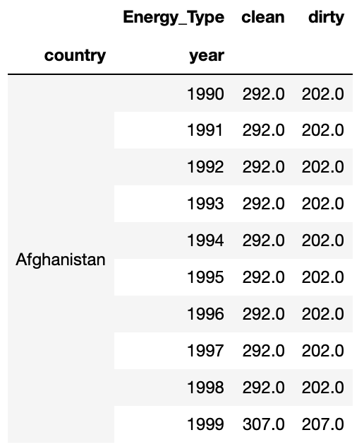
clean_vs_dirty = elec_df.pivot_table(values = 'quantity', index = ['country', 'year'], columns = 'Energy_Type', aggfunc = 'sum', fill_value = 0)

At this point my data looked like this:

Mapping Prepwork

For simplicity sake, I decided to add a marker of 1 if a country produced more clean energy than dirty energy (otherwise 0). This was accomplished with the following function and application:

def map_marker(df):
    marker = 0
    if df.clean >= df.dirty:
        marker = 1
    else:
        marker = 0
    return marker

clean_vs_dirty['map_marker'] = (clean_vs_dirty.clean >= clean_vs_dirty.dirty)*1

Next, I needed to add the proper codes for the countries that would correspond to mapping codes. I used the Alpha 3 Codes, which can be found here. I imported these codes as a dictionary and applied them to my Dataframe with the following code:

#The following line gives me the country name for every row
clean_vs_dirty.reset_index(inplace = True)

df_codes = pd.DataFrame(clean_vs_dirty.country.transform(lambda x: dict_alpha3[x]))
df_codes.columns = ['alpha3']
clean_vs_dirty['alpha3'] = df_codes

Great! Now I’m ready to map!

Mapping

I wanted to use a cool package I found called plotly.express. It is an easy way to create quick maps. I started with the 2014 map, which I accomplished with the following python code:

clean_vs_dirty_2014 = clean_vs_dirty[clean_vs_dirty.year == 2014]

import plotly.express as px
    
fig = px.choropleth(clean_vs_dirty_2014, locations="alpha3", color="map_marker", hover_name="country", color_continuous_scale='blackbody', title = 'Clean vs Dirty Energy Countries')
fig.show()

This code produced the following map, where blue shaded countries produce more clean energy than dirty energy and black shaded countries produce more energy through dirty sources than clean sources:

You can see here that many major countries, such as the US, China, and Russia were still producing more dirty energy than clean energy in 2014.

Year by Year Maps

As a fun next step, I decided to create a slider using the ipywidgets package to be able to cycle through the years of maps for energy production data. With the following code (and a little manual gif creation at the end) I was able to create the gif map output below, which shows how the countries have changed from 1992 to 2014.

def world_map(input_year):
    
    fig = px.choropleth(clean_vs_dirty[clean_vs_dirty.year == input_year], locations="alpha3", color="map_marker", hover_name="country", color_continuous_scale='blackbody', title = 'Clean vs Dirty Energy Countries')
    fig.show()

import ipywidgets as widgets
from IPython.display import display

year = widgets.IntSlider(min = 1992, max = 2014, value = 1990, description = 'year')

widgets.interactive(world_map, input_year = year)

Success!

I was able to create a meaningful representation of how countries are trending over time. Many countries in Africa, Europe, and South America are making improvements in their clean energy production. However, the US and other major countries were still too reliant on dirty energy as of 2014.